The Curious Case of Well-Behaved Matrices
A few days ago, a friend of mine suggested using "low-rank methods" in my neural-networks-from-scratch work, to showcase how basic concepts of linear algebra play an important role in neural networks. I started digging into the topic, and while surfing the internet, I stumbled upon a comment on Reddit saying, "initialize your weights orthogonally for better stable gradients".
The idea of orthogonally initialized weights is fascinating, but I couldn't find any good explanation stating why this method works — so I decided to cook up some math myself.
## 1. Understanding gradients
To understand how orthogonal initialization helps, I started analyzing the gradient matrix. I wrote the gradient equation and broke it into three major parts like this:
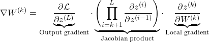
This scary-looking expression is nothing but a chain of matrix products, which helps in visualizing how gradients flow in neural networks:
- -The first term is the gradient of the loss with respect to the output of the last layer.
- -The middle term forms a sequence of Jacobian matrices, each representing how the output of one layer depends on the previous.
- -The last term is the local gradient — i.e. how the output of layer (l) depends on its own weights.
What matters here is the middle product of Jacobians, because it carries the gradient signal backward through the layers.
## 2. Analyzing jacobians
Considering a linear layer like this:

Its Jacobian will be written as:

Again, a scary-looking equation, but it's just simple calculus.
### Key observations from this equation
- -If I use ReLU as my activation, then its derivative will be either 0 or 1.
- -The Jacobian matrix is directly dependent on the weight matrix.
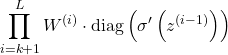
Thus, the product of Jacobian matrices in the first equation can be replaced by:
## 3. Expressing the gradient equation using matrix norms
Using the submultiplicative property of matrix norms on the gradient equation:

From the earlier equation, I rewrote the gradient equation by replacing the Jacobian matrix with the weight matrix like this:

## 4. Case 1: Gaussian initialization of weights
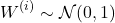
If I initialize weights with entries drawn i.i.d. from a normal distribution:
Then the spectral norm of the weight matrix will be:
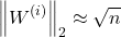
This is because:
- -The output of multiplying a vector with Gaussian (W) is just a weighted sum of n Gaussian columns.
- -Each component in such a product will be a Gaussian with variance 1.
- -Thus, the squared norm will be the expected value of a Gaussian, i.e. n.
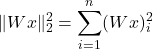
And thus we get:

In the equation from Expressing the Gradient Equation Using Matrix Norms, the spectral norm of the weight matrix will be replaced like this:
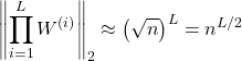
This will grow exponentially for (n > 1) and vanish quickly for (n < 1), and thus in turn affect the value of the gradient (as we proved earlier, gradient values directly depend upon the weight matrix).
## 5. Case 2: Orthogonal initialization
If we initialize weights orthogonally by using QR decomposition on weights sampled from a normal distribution, then we know that their singular values will be 1 because:

And thus, I can substitute this into the original gradient norm equations, resulting in:

As you can see, the gradients are stable and won't explode or vanish even if we have huge depth in our neural network.
## Thank god, the math works out
I modified my code from the last blog by increasing the layers and their widths, and initializing weights orthogonally using QR decomposition.
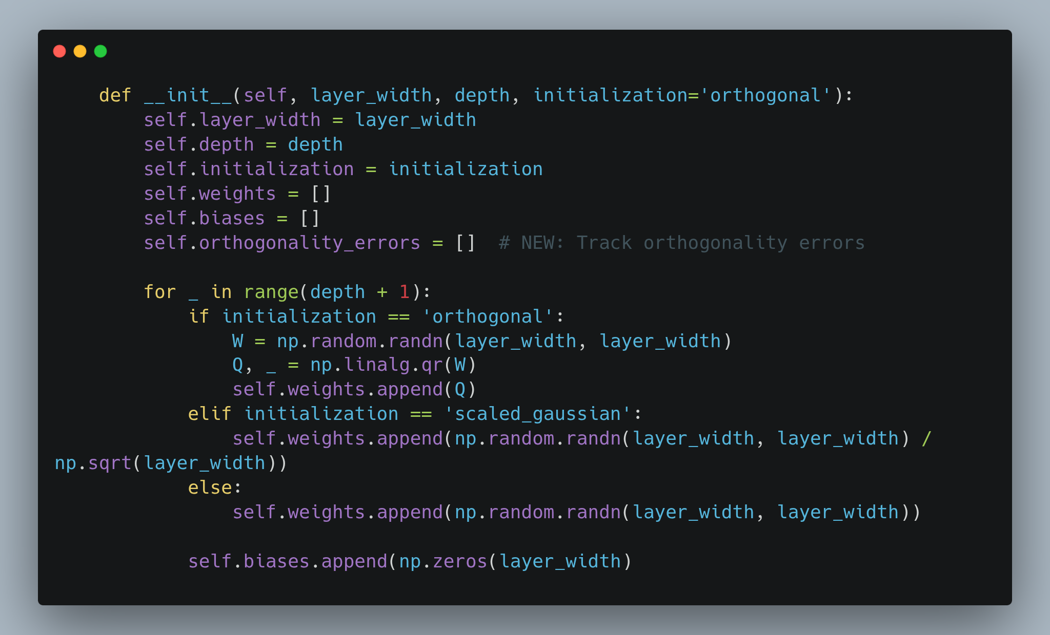
And it turns out that all the math I did till now works out (thank God!). I plotted the gradient norms vs. layer depth for Gaussian weights and orthogonal weights.
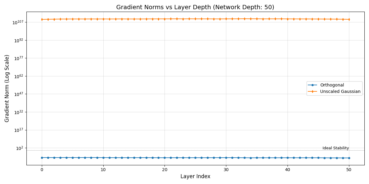
Clearly, for Gaussian-initialized weights the gradient norms explode, while for orthogonally-initialized weights the gradient norms stay within a good range.
(I generated synthetic data using np.rand for this.)
## But how are the weights orthogonal throughout training???
I tried to verify whether the weights stay orthogonal — or nearly orthogonal — by tracking them during backpropagation:
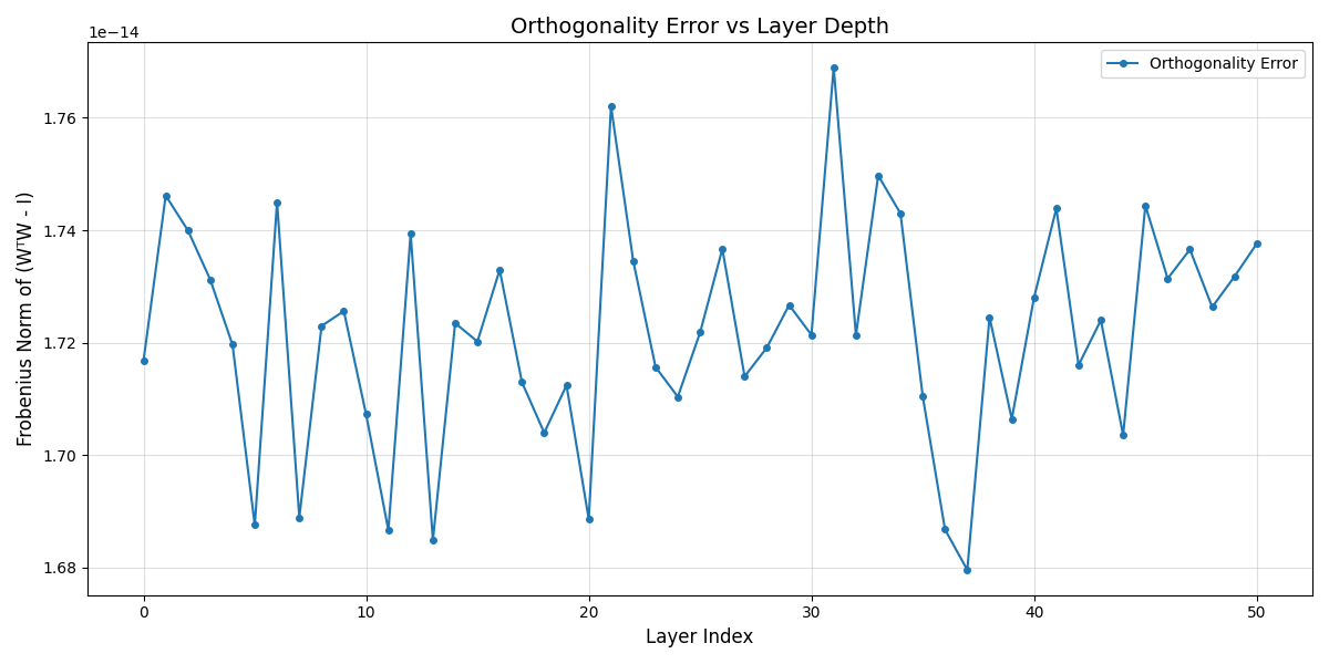
Even after working out the math and implementing everything, I still can't fully understand how the weights remain orthogonal or nearly orthogonal. Maybe a good topic for the next blog.
Hope you got some good insights from this!